This module wasn’t run in the 2026 CBW microbiome workshop, but we did run it in 2025. You can find those materials here.
Introduction
In this module, we’re going to be learning the basics of moving around on the command line, creating directories, zipping and unzipping folders, making tar archives and installing programs on a server. We’ll also be downloading files to the server, investigating the format of fasta and fastq files, and looking at the quality of sequenced samples.
Throughout this module, there are some questions aimed to help your understanding of some of the key concepts. You’ll find the answers at the bottom of this page.
Logging into a server
I’m going to skip most of this because it will vary so much depending on which server you are using. Hopefully, whoever set you up with access to a server will be able to give you directions on logging in for the first time. This will usually be from your Terminal, so go ahead and open up this program on your laptop.
The command you will need to use will vary a little, but it will usually look something like this:
ssh username@servername
In this case, when you press enter after typing this, you should be prompted for a password, which you will need to type in and press enter.
If it is your first time connecting, it will then probably ask you if you’re sure you want to connect. Type yes and press enter/
Or you may have been given a file with the extension .pem. Save this and go to where you’ve saved it in your finder/folders. Right click the file, hold the option key and click on “Copy CBW.pem as pathname”.
You can just remove the CBW.pem from the end to get the file path. E.g., my full path name that I copied is /Users/robynwright/Downloads/CBW.pem, so:
cd /Users/robynwright/Downloads
Then run:
chmod 600 CBW.pem
Make sure that you replace CBW.pem with whatever the file name is that you saved it as!
Now we can connect to the server:
ssh -i CBW.pem ubuntu@##.uhn-hpc.ca
Note that this is the server name used in the CBW workshops. If you are outside of this, your server address will likely look different!
If it is your first time connecting, it will then probably ask you if you’re sure you want to connect. Type yes and press enter/
Whichever method you used for logging in, hopefully your screen looks something like this afterwards: 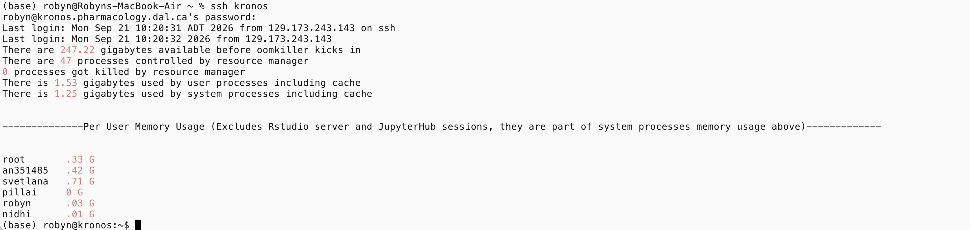
1. Creating directories and moving around on the command line
Now that we’re logged in, we’re going to get familiar with what’s on the server. First of all, type ls and press enter. If it is your first time on a server, this will likely be empty, but if anything is here then these will be your folders.
Think of these like you would the directories on your own computer, e.g. My Documents and Downloads, and this first folder is just like looking in /home/users/yourname/ on your own computer. The ls command is just telling the server to list out the files/directories in the directory that we’re currently in.
Next, type in pwd and press enter. The pwd command tells you which directory you’re currently in. I am in /home/robyn and yours will likely look similar!
Now, we will want to create a directory to work in. Type in mkdir microbiome_tutorial and press enter. If you type in ls again, you should see now that you have a new folder called microbiome_tutorial.
Now we’re going to change directory. We can change to any directory that exists here, but we’ll change to the one we just made. Type in cd microbiome_tutorial and press enter (you will always need to press enter to run a command). If you type in pwd again, you should see that you’ve changed directory. If you type in ls, you should see that the directory is empty.
Now what happens if we want to go back to our first directory? We can use cd .., which will take us up one level. Try that and then use the ls command again. You should see the folder that you made. If you use cd on it’s own, then it’ll take you back to where you started. Try it and then use the pwd command.
Note that any time you log out from the server (or lose connection/time out and get logged out), you will need to change back to the directory that you’re working from. Go back to the directory we made: cd microbiome_tutorial
Use the pwd command once more to check that you’re in the right place
2. Use wget to download files
Now we’re going to download some files to use. There are a lot of different data repositories available online, but we’re going to use some data from the Human Microbiome Project. This repository is quite straightforward because all we need is a link to the data and we can download it, but other repositories require their own programs and file formats for downloading which can make them quite complicated (and frustrating, if you don’t know what you’re doing!) to use. You can see the webpage that we’re taking the files from here.
Now we’ll download the files. There are a few different commands that we can use for downloading files, so you might have seen others, or may see others in the future, but for now we’ll be using a command called wget. If you just type in wget on its own then you should see some information about it. You’ll see that it gives an error message, because we haven’t also given it a URL, but it also tells us that we can run wget --help to see more options. Try running that. If you scroll back up to where you ran it, you’ll see a huge list of options that you could give wget depending on what you want to do. We won’t be using most of these options for now, but you can usually add --help to whatever command you are trying to run to get some more information about what information it is expecting from you (these are called “arguments”).
We’re going to download three files like so:
wget https://g-227ca.190ebd.75bc.data.globus.org/ibdmdb/raw/HMP2/16S/2018-01-08/206534.fastq.gz
wget https://g-227ca.190ebd.75bc.data.globus.org/ibdmdb/raw/HMP2/16S/2018-01-08/206536.fastq.gz
wget https://g-227ca.190ebd.75bc.data.globus.org/ibdmdb/raw/HMP2/16S/2018-01-08/206538.fastq.gz
Remember that you need to press enter to run these!
You should see some progress bars come up, but these files aren’t very big so they shouldn’t take very long to download. Now use ls again to see the files. You should see:
206534.fastq.gz 206536.fastq.gz 206538.fastq.gz
3. Move these files to the directories
When we downloaded these, we didn’t make a directory to put them in, so let’s do that now so that we can tidy them up a bit:
mkdir test_data
And then we can move them to this directory we’ve just made using the mv command. The mv command is expecting the name of the file that we want to move, and then the directory/path that we want to move this file to as arguments:
mv 206534.fastq.gz test_data/
If you use the ls command again now, you will see that there’s only two files (along with the test_data directory). You can also use the ls command on the test_data directory: ls test_data, and you should see the file that we moved into there.
Often, we might have a lot of files to move and we don’t want to have to move them one by one. If we want to move multiple files of the same type, we can do that like this:
mv *.fastq.gz test_data/
The asterisk (*) acts as a wildcard, and anything that ends in .fastq.gz will be moved using this command. If you take a look in test_data again using the ls command, you should see all three files in there now, and not in your current directory. Another useful thing that you can do with the ls command is add another argument to get some information about the files: ls -lh test_data/. When you run this, you should see who has permission to read/write to the files, the author and the owner of the files, the size of the files, and when they were created. The -l is what is telling this to give you the information, and adding the h converts this into “human” readable format. Try using it without the h - you’ll see that the file sizes are in bytes instead of megabytes (MB/M).
4. Zip and unzip these files
You might have noticed the .gz on the end of the files indicating that they’re zipped (or compressed). Sometimes when we run bioinformatics programs they can uncompress the files within the program, but other times we need to uncompress (unzip) them first. These are quite small files so you might think it’s unnecessary to zip/compress them, but often we have thousands of sequencing data files and they can each be hundreds of gigabytes (GB) or even terabytes (TB) in size, so it becomes quite important to keep them compressed until we need them.
We’ll use the gunzip command to unzip them. Try typing in gunzip test_data/20 and then pressing the tab button. If you press it a couple of times, you should see a list of your options come up. The tab button can be really useful for completing file paths for you and saving you a lot of typing! Continue typing and choose one of the files to unzip (e.g. type in 8 and then press tab again and then enter). Now if you run ls -lh test_data again, you should see that the file you unzipped no longer has the .gz on the end, and it’s much larger in size now.
We’ll zip the file back up for now: gzip test_data/20 - if you press tab to complete again (and enter), you should find that this will auto-fill with the file that you unzipped, because it’s the only file type that the command is able to work with.
What happens if you try to run this on a file that is already zipped? gzip test_data/206538.fastq.gz It should tell you that it’s unable to run because .gz is already on that file.
Let’s unzip all of the files now: gunzip test_data/* See that we can use the asterisk (*) again as a wildcard and it will unzip every file in the test_data directory. Take a look at the directory with ls or ls -lh if you like. Remember to add the directory name!
5. Create new tar archive of files
There are several different ways of compressing files - there is gzip/gunzip that we just used, but we can also package up multiple files inside a directory together. We’ll be using the tar command for this, and as you can see if you run tar --help, you’ll see that there are lots of options available for this. Let’s try it out with the test_data directory: tar -czvf test_data.tar.gz test_data/
Here we gave the command several arguments: -czvf (see below), test_data.tar.gz (the file name that we want our tar archive to have) and test_data/ (the name of the directory that we want to compress.
-czvf is a short way of giving several arguments to the command: c for “create” (creates a new archive), z for “gZip” (this tells tar to write/read through gzip), v stands for “verbose” (meaning that it will print out information about what it is doing), and f for “file” or “archive”.
If you now run ls -lh, you should see that the tar archive (test_data.tar.gz) is a smaller size than the 3 files would be together (check by running ls -lh test_data). You can also take a look at what’s in the tar archive with the less command: less test_data.tar.gz. Press q (for “quit”) when you’re ready to exit.
Usually we’ll make a tar archive because we want to keep our files but save some space, so let’s delete the original folder: rm -r test_data/. Hopefully by now you’re getting the hang of how these commands work. The rm command is for removing files - you should always be really careful when using it because it won’t ask you if you’re sure like your regular computer would, and most servers don’t have a “recycle bin” for the files to be sent to, so if you remove them, they’re gone for good. The -r argument is for removing a directory rather than just a file.
6. Unzip tar archive
If we need to use the data that we zipped into the tar archive again, we’ll need to unzip - or extract - it.
To unzip the tar archive, we can do that like so: tar -xvf test_data.tar.gz. Note that we just replaced the cz with x for “eXtract”. You should be able to see the files back in test_data with the ls command.
7. Look at fasta and fastq files with less
Now we’re going to take a look at these files. Let’s look at 206538 first: less test_data/206538.fastq. You can scroll through the file, and remember to press q when you want to stop looking at the file. If you want to look at it again, press the up arrow key to run the less command again. You can always press the up arrow to go back through the commands that you’ve run previously. If you’ve typed something wrong and want to start again, press ctrl+c to get back to a blank command prompt.
You should have noticed that this file had the .fastq extension. Let’s copy across the same files in fasta format from our lab server:
wget https://kronos.pharmacology.dal.ca:8080/public_files/MH2/unix_tutorial/test_data_fasta.tar.gz
And extract this tar file:
tar -xvf test_data_fasta.tar.gz
Take a look at the same file in fasta format: less test_data_fasta/206538.fasta
You can also download these files using the scp (server copy) command to copy them across to your own computer. This is a really useful command that you will likely use a lot! You won’t always want to copy across files if they are too big, but you will often want to download the end result of your analyses, or download intermediates to open up and help you with trouble-shooting when you run into issues.
You would do that by going to a new Terminal window/tab. Navigate to the location that you would like to save the files to (using cd as we did above). To download the whole folder, you can run:
scp -r robyn@kronos.pharmacology.dal.ca:/home/robyn/microbiome_tutorial/test_data_fasta/ .
scp -r robyn@kronos.pharmacology.dal.ca:/home/robyn/microbiome_tutorial/test_data/ .
Note that here the -r argument is the same as above for rm - it means that we’re taking a directory and not a file, and then the . shows that we want to copy the data into the directory that we are currently in. We could replace it with another file path if we wanted.
It’s also important to see that you’re giving the full server address that you would have used for logging in with ssh (robyn@kronos.pharmacology.dal.ca for me), followed by :/, and then giving the full file path that you would get with pwd.
If you were using a .pem file (as in the CBW workshops), this command would look like this:
scp -i CBW.pem -r ubuntu@##.uhn-hpc.ca:/home/ubuntu/workspace/bmb_module1/test_data_fasta/ .
scp -i CBW.pem -r ubuntu@##.uhn-hpc.ca:/home/ubuntu/workspace/bmb_module1/test_data/ .
Now you can open the files with a text editor like TextEdit (Mac) or Notepad (Windows). You should see that the fastq file has 4 lines for each sequence, while the fasta only has two. The fasta has a first line that starts with > that contains the sequence name and description, and the second line contains the actual DNA sequence (DNA in this case, but this file format could also contain RNA or protein sequences). fastq files start the same, with the first line containing the sequence name and description (but starting with an @ symbol instead), and the second containing the sequence. The third line then contains a + character, and the fourth contains quality information about each base of the sequence (and should contain the same number of characters as the sequence). You can read more about the quality information that the symbols encode here.
To count the number of lines in a file, we can use the less command again, with some additional information: less test_data/206538.fastq | wc -l
Here, the | means that we are giving another command, the wc stands for word count, and the -l means we are counting the number of lines.
You should see that this file contains 63,048 lines.
Question 1: How many sequences does this mean that there are?
Remember that you can just use less test_data/206538.fastq to look at the file.
Now do the same for the fasta file: less test_data_fasta/206538.fasta | wc -l.
You should see that the fasta file contains half the number of lines as the fastq file. Sometimes you’ll find that the sequences with a fasta file are split across multiple lines, in which case, simply counting the number of lines wouldn’t work, so there are also other ways to count the number of sequences in a file, and these can be adapted for other purposes, too. E.g.: grep -c ">" test_data_fasta/206538.fasta - the grep command pulls out every occurrence of a phrase (or string, as it’s usually called in programming) and the -c argument tells it to count these. What happens if you don’t use the -c argument? Why do you think this happened?
In most programming languages, you have positional arguments and named arguments. Positional arguments need to be included in the proper position, or order. The order of positional arguments is defined within the program. Named or keyword arguments are given or passed to the program only after the name is given. In the case above, the -c ">" is a named argument and the file name test_data_fasta/206538.fasta is a positional argument.
Question 2: What happens if you try to do the same thing with@for the fastq file? Why is this?
Remember to look at the fastq file with the less command for clues, or try running it without the -c argument.
8. Installing programs to the server
Now we’re going to learn how to install programs to the server. A lot of the commands we have just used (like grep and less) are standard ones that will be installed on most servers, but frequently we will need to install other programs (usually called packages), too. The packages that we use are often not as stable as those that we download and use on our laptops (like Microsoft Word or Adobe Acrobat Reader) and so they sometimes depend on a particular version of another package. It frequently takes more time to install packages than it does to run them, and any bioinformatician will tell you how frustrating it can be. Anaconda can help to manage this, although it doesn’t overcome these problems entirely!
You can download Anaconda like so:
curl -O https://repo.anaconda.com/archive/Anaconda3-2026.07-1-Linux-x86_64.sh
Note that if you are not running a Linux server, you may want to find a different download link and modify the subsequent commands!
And then:
bash Anaconda3-2026.07-1-Linux-x86_64.sh
#hold down enter key until you get to the end of the agreement, or press q
#type yes
#confirm location by pressing enter
#yes
#now close and reopen the window - you'll need to log back in the same way as you did before!
9. Conda environments
Anaconda, or conda, allows us to have separate “environments” for installing packages into. This means that if one package requires version 3.1 of another package, but another requires version 2.9, they won’t interfere with each other. Often when we’re installing new packages or starting a new project, we’ll make a new environment. This also helps us to keep track of which versions of a package we’ve used for a specific project. The environment is essentially a directory that contains a collection of packages that you’ve installed, so that other packages know where to access the package that they need to use. We’re going to make a new environment to install some packages into:
conda create -n tutorial
You’ll see that here we’re using the conda command first, and then giving it the create and -n tutorial arguments. We could call this environment anything we like, but it’s best to make this descriptive of what it is so that when we collaborate with others or share our code, it’ll be obvious what this environment is for.
You’ll need to press y at some point, to confirm that you want to install new packages.
Now we can “activate” this environment like this: conda activate tutorial. Any time you are logged out and you log back in, you’ll need to reactivate the environment if you want to be working from it. If you want to see the other environments that are installed and available, you can run conda info --envs. In the next step of the tutorials, I give you instructions on installing all of the packages that you’ll need.
10. Install fastqc and multiqc
Now we’ll install the packages that we want to use. Usually if there’s a package that you’re interested in, for example we’ll be using one called fastqc, you can just google conda install fastqc and you should see an anaconda.org page as one of the top hits, telling you how to install it. Sometimes you’ll also see bioconda documentation, or a package recipe and this might give more details if you’re struggling to install it. We’ll install fastqc like this:
conda install bioconda::fastqc
You’ll need to confirm that you want to install things with y at some point. If you forgot to activate the environment (see above), then you may get an error that you don’t have permissions to do this!
You can test to see whether it got installed by typing which fastqc - this should show you the location that it’s installed in, and it should be something like: /opt/anaconda3/envs/tutorial/bin/fastqc.
Now we’ll install the second package that we need:
conda install bioconda::multiqc
Confirm this again with y
As you might have guessed from the qc in both of these names, we’ll be using them for Quality Control of the sequence data.
11. Perform quality control on fastq files
First we’ll be running fastqc, and to do that, we’ll first make a directory for the output to go: mkdir fastqc_out
Now we’ll run fastqc:
fastqc -t 4 test_data/*.fastq -o fastqc_out
Here the arguments that we’re giving fastqc are:
-t 4: the number of threads to use. Sometimes “threads” will be shown as--threads,--cpus,--processors,--nproc, or similar. Basically, developers of packages can call things whatever they like, but you can use the help documentation to see what options are available. We’re using 4 here because that’s the maximum that is available on the Amazon servers used for the microbiome workshops. See below (htop) for how we find out about how many we have available.test_data/*.fastq: the fastq files that we want to check the quality of.-o fastqc_out: the folder to save the output to.
12. htop - looking at the number of processes we have available or running
Try running htop. This is an interactive viewer that shows you the processes that are running on your computer/server. There are a lot of different bits of information that this is showing us - you can see all of that here. Yours will look slightly different, but I’ll give some information based on mine and hopefully you can apply this to yours!
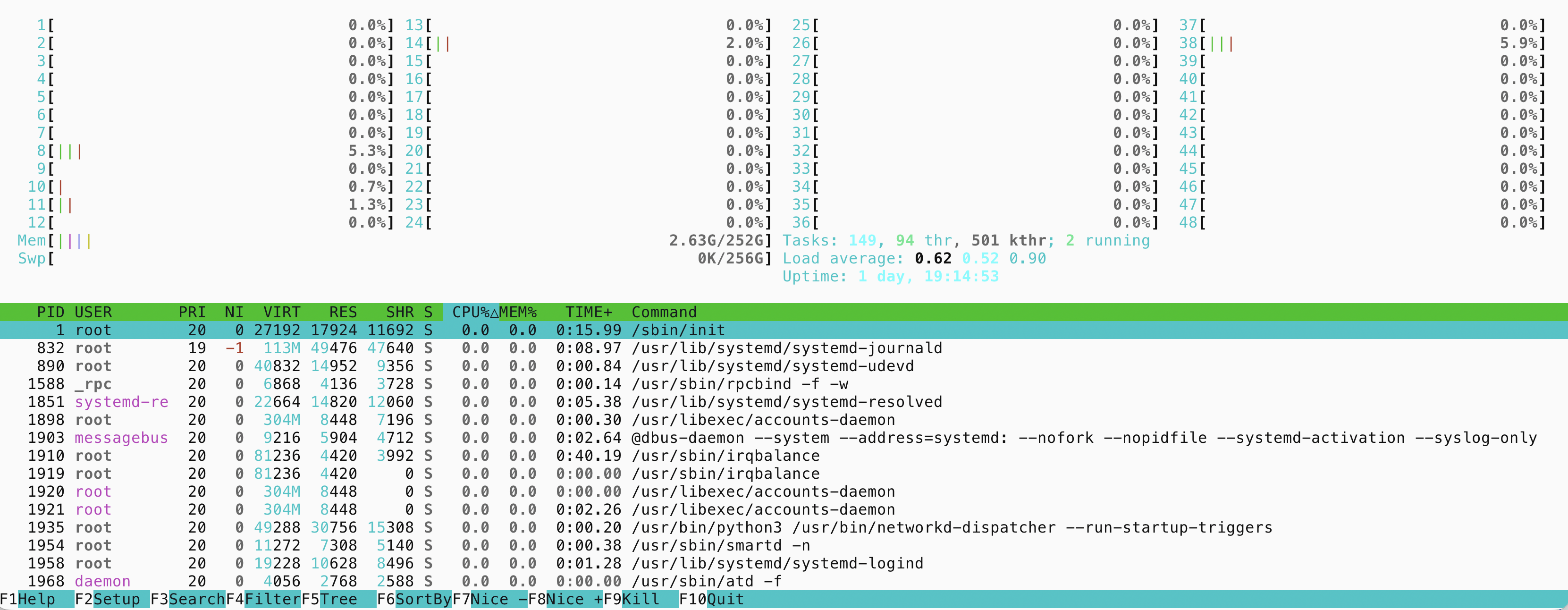
The CPUs(labelled 0-48 at the top) - this shows the percentage of the CPU being used for each core, and the number of cores shown here is the number of different processes/threads that we have available to us. In our case, this is 48.Memory- this is the amount of memory, or RAM, that we have available to us. You’ll see that it is 252GB - this is pretty decent for bioinformatics analysis, although our other server has ~1.5 TB. Hopefully your server for bioinformatics will have much more than a standard computer! The larger your dataset, or the deeper your sequencing depth, the more RAM you are likely to need.The processes(at the bottom) - you can see everything that is running under aPID(Process ID). This is useful when you’re using a shared server to see who is running what, particularly for when you’re wanting to run something that will use a lot of memory or will take a long time and you want to check that it won’t bother anyone else.
When you’re done looking at this, press F10 (on a Mac this is fn+F10) or q to exit from this screen.
13. Back to the quality control
Now take a look at one of the .html files in fastqc_out. You’ll need to download it as you did above!
scp -r robyn@kronos.pharmacology.dal.ca:/home/robyn/microbiome_tutorial/fastqc_out/ .
Next we’ll run multiqc. The name suggests it might be performing QC on multiple files, but it’s actually for combining the output together of multiple files, so we can run it like this:
multiqc fastqc_out --filename multiqc.html
So we’ve given as arguments:
fastqc_out: the folder that contains the fastqc output.--filename multiqc.html: the file name to save the output as.
Now look at multiqc.html (copy it across using scp as you did above!).
There are some questions here to help you look at the files and interpret these:
Question 3: What is the GC% of the samples?
Question 4: What % of the samples are duplicate reads? Is this what you expected?
Question 5: Now look at the Sequence Counts section. Which sample has the most reads?
Question 6: How many unique and duplicate reads are in sample 206536?
Question 7: Look at the Sequence Quality Histograms. Do these seem good to you? Why or why not? Does this seem normal?
Question 8: Look at the top overrepresented sequence. If you want to see what it is, paste it into the “Enter accession number(s), gi(s), or FASTA sequence(s)” box here and click on the blue “BLAST” button at the bottom of the page.
Answers
Question 1: How many sequences does this mean that there are? Remember that you can just use less test_data/206538.fastq to look at the file.
Each sequences is spread across four different lines, so there are 63,048/4 = 15,762 sequences.
Question 2: What happens if you try to do the same thing with @ for the fastq file? Why is this? Remember to look at the fastq file with the less command for clues, or try running it without the -c argument.
The number of @ in the fastq file is much more than the number of lines. This is because the @ symbol is also used in the quality information. We can get round this by using part of the sample name, e.g., grep -c "@206534" test_data/206534.fastq.
Question 3: What is the GC% of the samples?
51%
Question 4: What % of the samples are duplicate reads? Is this what you expected?
In the “General Statistics” section, we can see that ~97% of the reads are duplicated. Looking in the “Sequence Counts” section and hovering over each sample will show us how many of the reads are unique. This makes sense, because the reads are from PCR-amplified samples so we are expecting most to occur more than once.
Question 5: Now look at the Sequence Counts section. Which sample has the most reads?
206354.
Question 6: How many unique and duplicate reads are in sample 206536?
752 and 29,883.
Question 7: Look at the Sequence Quality Histograms. Do these seem good to you? Why or why not? Does this seem normal?
The sequence quality here is all really high! These are all good sequences, but this isn’t normal. This is because the samples that are available for download from the HMP website have already been quality filtered.
Question 8: Look at the top overrepresented sequence. If you want to see what it is, paste it into the “Enter accession number(s), gi(s), or FASTA sequence(s)” box here and click on the blue “BLAST” button at the bottom of the page.
All of the top hits are Bacteroides (finegoldii, caccae, stercoris, etc). These samples are from HMP2 IBD gut samples, so this seems normal!
Authors
Author: Robyn Wright
Modifications by: NA
Based on initial versions by: NA